Getting started with INTEGRATE - posterior analysis only¶

This notebook contains a simple example of getting started with INTEGRATE - analyzing the posterior only.

Load the the results of inversion
Plot some results

[1]:

try:
    # Check if the code is running in an IPython kernel (which includes Jupyter notebooks)
    get_ipython()
    # If the above line doesn't raise an error, it means we are in a Jupyter environment
    # Execute the magic commands using IPython's run_line_magic function
    get_ipython().run_line_magic('load_ext', 'autoreload')
    get_ipython().run_line_magic('autoreload', '2')
except:
    # If get_ipython() raises an error, we are not in a Jupyter environment
    # # # # #%load_ext autoreload
    # # # # #%autoreload 2
    pass

[2]:

import integrate as ig
# check if parallel computations can be performed
parallel = ig.use_parallel(showInfo=1)
hardcopy = True
import matplotlib.pyplot as plt

Notebook detected. Parallel processing is OK.

0. Get some TTEM data¶

A number of test cases are available in the INTEGRATE package To see which cases are available, check the get_case_data function

The code below will download the file DAUGAARD_AVG.h5 that contains a number of TTEM soundings from DAUGAARD, Denmark. It will also download the corresponding GEX file, TX07_20231016_2x4_RC20-33.gex, that contains information about the TTEM system used.

[3]:

case = 'DAUGAARD'
files = ig.get_case_data(case=case,  loadType='post')
f_data_h5 = files[0]
f_post_h5 = files[-1]
f_prior_h5 = files[3]
file_gex= ig.get_gex_file_from_data(f_data_h5)


print("Using data file: %s" % f_data_h5)
print("Using GEX file: %s" % file_gex)
print("Using prior in file: %s" % f_prior_h5)
print("Using posterior in file: %s" % f_post_h5)

Getting data for case: DAUGAARD
--> Got data for case: DAUGAARD
Using data file: DAUGAARD_AVG.h5
Using GEX file: TX07_20231016_2x4_RC20-33.gex
Using prior in file: README_DAUGAARD
Using posterior in file: POST_DAUGAARD_AVG_prior_detailed_general_N2000000_dmax90_TX07_20231016_2x4_RC20-33_Nh280_Nf12_Nu2000000_aT1.h5

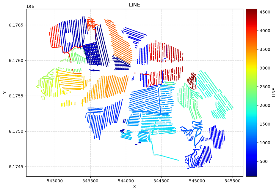
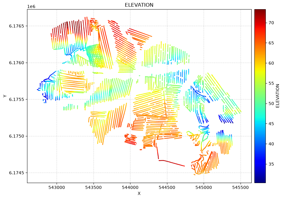
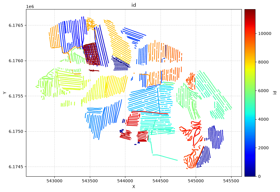
Plot the geometry and the data¶

ig.plot_geometry plots the geometry of the data, i.e. the locations of the soundings. ig.plot_data plots the data, i.e. the measured data for each sounding.

[4]:

# The next line plots LINE, ELEVATION and data id, as three scatter plots
# ig.plot_geometry(f_data_h5)
# Each of these plots can be plotted separately by specifying the pl argument
ig.plot_geometry(f_data_h5, pl='LINE')
ig.plot_geometry(f_data_h5, pl='ELEVATION')
ig.plot_geometry(f_data_h5, pl='id')

f_data_h5=DAUGAARD_AVG.h5
f_data_h5=DAUGAARD_AVG.h5
f_data_h5=DAUGAARD_AVG.h5

../_images/notebooks_integrate_getting_started_posterior_only_6_1.png

../_images/notebooks_integrate_getting_started_posterior_only_6_2.png

../_images/notebooks_integrate_getting_started_posterior_only_6_3.png

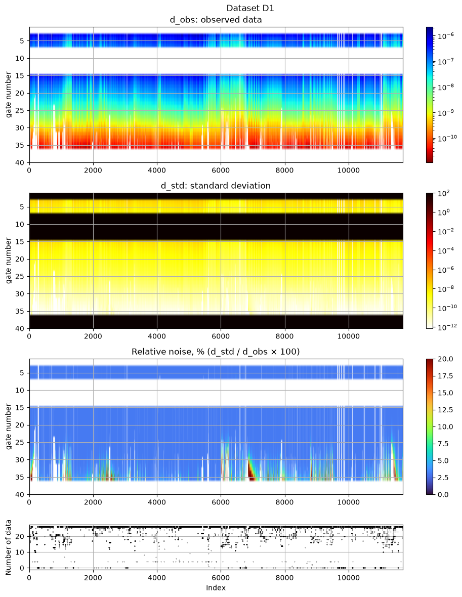
[5]:

# The data, d_obs and d_std, can be plotted using ig.plot_data
ig.plot_data(f_data_h5, hardcopy=hardcopy)

../_images/notebooks_integrate_getting_started_posterior_only_7_0.png

1. Setup the prior model ($:nbsphinx-math:rho`(:nbsphinx-math:mathbf{m}`,:nbsphinx-math:mathbf{d}))¶

In this case prior data and models are allready available in the HDF% in ‘f_prior_h5’.

[6]:

# Plot some summary statistics of the prior model, to QC the prior choice
ig.plot_prior_stats(f_prior_h5, hardcopy=hardcopy)

---------------------------------------------------------------------------
OSError                                   Traceback (most recent call last)
Cell In[6], line 2
      1 # Plot some summary statistics of the prior model, to QC the prior choice
----> 2 ig.plot_prior_stats(f_prior_h5, hardcopy=hardcopy)

File ~/space/PROGRAMMING/integrate_module/integrate/integrate_plot.py:3673, in plot_prior_stats(f_prior_h5, Mkey, nr, use_log, showInfo, im, **kwargs)
   3670 import matplotlib.pyplot as plt
   3671 from matplotlib.colors import LogNorm
-> 3673 with h5py.File(f_prior_h5,'r') as f_prior:
   3674
   3675     # Convert im to Mkey if provided
   3676     if im is not None and len(Mkey) == 0:
   3677         Mkey = 'M%d' % im

File ~/space/PROGRAMMING/integrate_module/.venv/lib/python3.12/site-packages/h5py/_hl/files.py:555, in File.__init__(self, name, mode, driver, libver, userblock_size, swmr, rdcc_nslots, rdcc_nbytes, rdcc_w0, track_order, fs_strategy, fs_persist, fs_threshold, fs_page_size, page_buf_size, min_meta_keep, min_raw_keep, locking, alignment_threshold, alignment_interval, meta_block_size, track_times, **kwds)
    546     fapl = make_fapl(driver, libver, rdcc_nslots, rdcc_nbytes, rdcc_w0,
    547                      locking, page_buf_size, min_meta_keep, min_raw_keep,
    548                      alignment_threshold=alignment_threshold,
    549                      alignment_interval=alignment_interval,
    550                      meta_block_size=meta_block_size,
    551                      **kwds)
    552     fcpl = make_fcpl(track_order=track_order, track_times=track_times,
    553                      fs_strategy=fs_strategy, fs_persist=fs_persist,
    554                      fs_threshold=fs_threshold, fs_page_size=fs_page_size)
--> 555     fid = make_fid(name, mode, userblock_size, fapl, fcpl, swmr=swmr)
    557 if isinstance(libver, tuple):
    558     self._libver = libver

File ~/space/PROGRAMMING/integrate_module/.venv/lib/python3.12/site-packages/h5py/_hl/files.py:232, in make_fid(name, mode, userblock_size, fapl, fcpl, swmr)
    230     if swmr:
    231         flags |= h5f.ACC_SWMR_READ
--> 232     fid = h5f.open(name, flags, fapl=fapl)
    233 elif mode == 'r+':
    234     fid = h5f.open(name, h5f.ACC_RDWR, fapl=fapl)

File h5py/_objects.pyx:54, in h5py._objects.with_phil.wrapper()
---> 54 'Could not get source, probably due dynamically evaluated source code.'

File h5py/_objects.pyx:55, in h5py._objects.with_phil.wrapper()
---> 55 'Could not get source, probably due dynamically evaluated source code.'

File h5py/h5f.pyx:106, in h5py.h5f.open()
--> 106 'Could not get source, probably due dynamically evaluated source code.'

OSError: Unable to synchronously open file (file signature not found)

It can be useful to compare the prior data to the observed data before inversion. If there is little to no overlap of the observed data with the prior data, there is little chance that the inversion will go well. This would be an indication of inconsistency. In the figure below, one can see that the observed data (red) is clearly within the space of the prior data.

[7]:

ig.plot_data_prior(f_prior_h5,f_data_h5,nr=1000,hardcopy=hardcopy)

---------------------------------------------------------------------------
OSError                                   Traceback (most recent call last)
Cell In[7], line 1
----> 1 ig.plot_data_prior(f_prior_h5,f_data_h5,nr=1000,hardcopy=hardcopy)

File ~/space/PROGRAMMING/integrate_module/integrate/integrate_plot.py:3104, in plot_data_prior(f_prior_data_h5, f_data_h5, nr, id, id_data, d_str, alpha, ylim, **kwargs)
   3100     id_data = id
   3102 cols=['wheat','black','red']
-> 3104 with h5py.File(f_data_h5,'r') as f_data, h5py.File(f_prior_data_h5,'r') as f_prior_data:
   3105
   3106     # Get data dimensions to determine plot type
   3107     prior_data = None
   3108     obs_data = None

File ~/space/PROGRAMMING/integrate_module/.venv/lib/python3.12/site-packages/h5py/_hl/files.py:555, in File.__init__(self, name, mode, driver, libver, userblock_size, swmr, rdcc_nslots, rdcc_nbytes, rdcc_w0, track_order, fs_strategy, fs_persist, fs_threshold, fs_page_size, page_buf_size, min_meta_keep, min_raw_keep, locking, alignment_threshold, alignment_interval, meta_block_size, track_times, **kwds)
    546     fapl = make_fapl(driver, libver, rdcc_nslots, rdcc_nbytes, rdcc_w0,
    547                      locking, page_buf_size, min_meta_keep, min_raw_keep,
    548                      alignment_threshold=alignment_threshold,
    549                      alignment_interval=alignment_interval,
    550                      meta_block_size=meta_block_size,
    551                      **kwds)
    552     fcpl = make_fcpl(track_order=track_order, track_times=track_times,
    553                      fs_strategy=fs_strategy, fs_persist=fs_persist,
    554                      fs_threshold=fs_threshold, fs_page_size=fs_page_size)
--> 555     fid = make_fid(name, mode, userblock_size, fapl, fcpl, swmr=swmr)
    557 if isinstance(libver, tuple):
    558     self._libver = libver

File ~/space/PROGRAMMING/integrate_module/.venv/lib/python3.12/site-packages/h5py/_hl/files.py:232, in make_fid(name, mode, userblock_size, fapl, fcpl, swmr)
    230     if swmr:
    231         flags |= h5f.ACC_SWMR_READ
--> 232     fid = h5f.open(name, flags, fapl=fapl)
    233 elif mode == 'r+':
    234     fid = h5f.open(name, h5f.ACC_RDWR, fapl=fapl)

File h5py/_objects.pyx:54, in h5py._objects.with_phil.wrapper()
---> 54 'Could not get source, probably due dynamically evaluated source code.'

File h5py/_objects.pyx:55, in h5py._objects.with_phil.wrapper()
---> 55 'Could not get source, probably due dynamically evaluated source code.'

File h5py/h5f.pyx:106, in h5py.h5f.open()
--> 106 'Could not get source, probably due dynamically evaluated source code.'

OSError: Unable to synchronously open file (file signature not found)

2. Sample the posterior $\sigma(\mathbf{m})$¶

The posterior distribution has allready been sampled using the extended rejection sampler.

3. Plot some statistics from $\sigma(\mathbf{m})$¶

Prior and posterior data¶

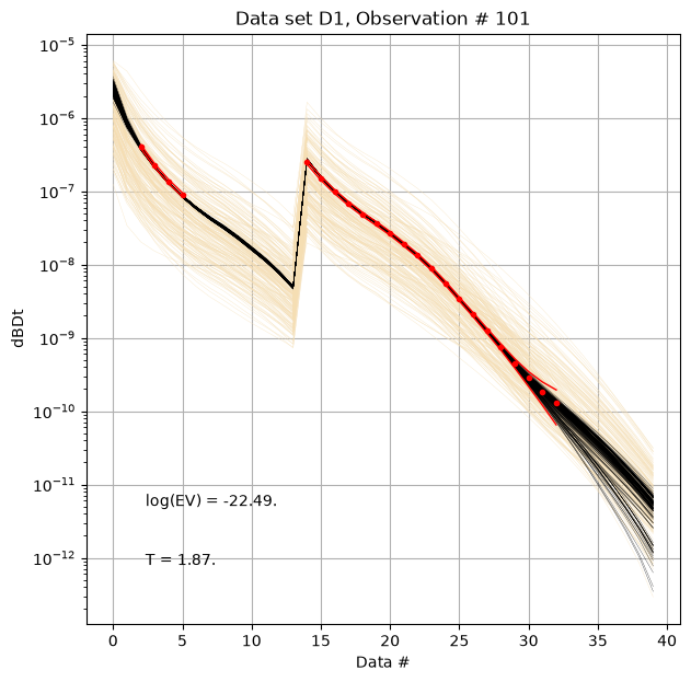
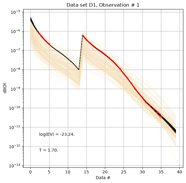
First, compare prior (beige) to posterior (black) data, as well as observed data (red), for two specific data IDs.

[8]:

ig.plot_data_prior_post(f_post_h5, i_plot=100,hardcopy=hardcopy)
ig.plot_data_prior_post(f_post_h5, i_plot=0,hardcopy=hardcopy)

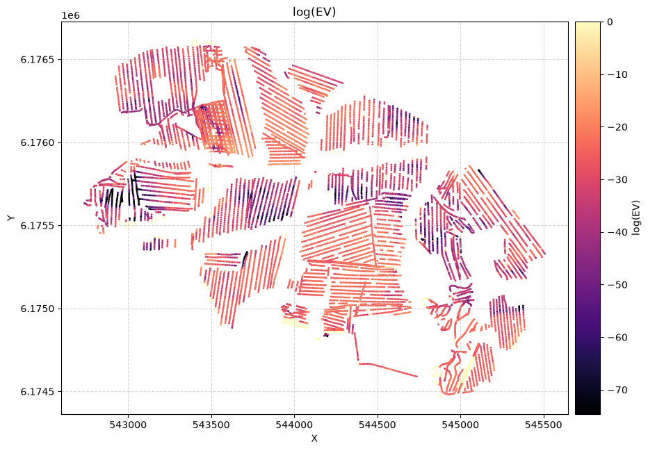
../_images/notebooks_integrate_getting_started_posterior_only_14_0.png

../_images/notebooks_integrate_getting_started_posterior_only_14_1.png

Evidence and Temperature¶

[9]:

# Plot the Temperature used for inversion
ig.plot_T_EV(f_post_h5, pl='T',hardcopy=hardcopy)
# Plot the evidence (prior likelihood) estimated as part of inversion
ig.plot_T_EV(f_post_h5, pl='EV',hardcopy=hardcopy)

Figure saved to POST_DAUGAARD_AVG_prior_detailed_general_N2000000_dmax90_TX07_20231016_2x4_RC20-33_Nh280_Nf12_Nu2000000_aT1_1_11693_T.png

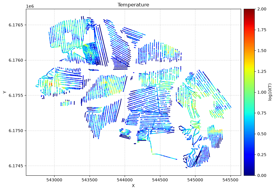
../_images/notebooks_integrate_getting_started_posterior_only_16_1.png

Figure saved to POST_DAUGAARD_AVG_prior_detailed_general_N2000000_dmax90_TX07_20231016_2x4_RC20-33_Nh280_Nf12_Nu2000000_aT1_1_11693_EV.png

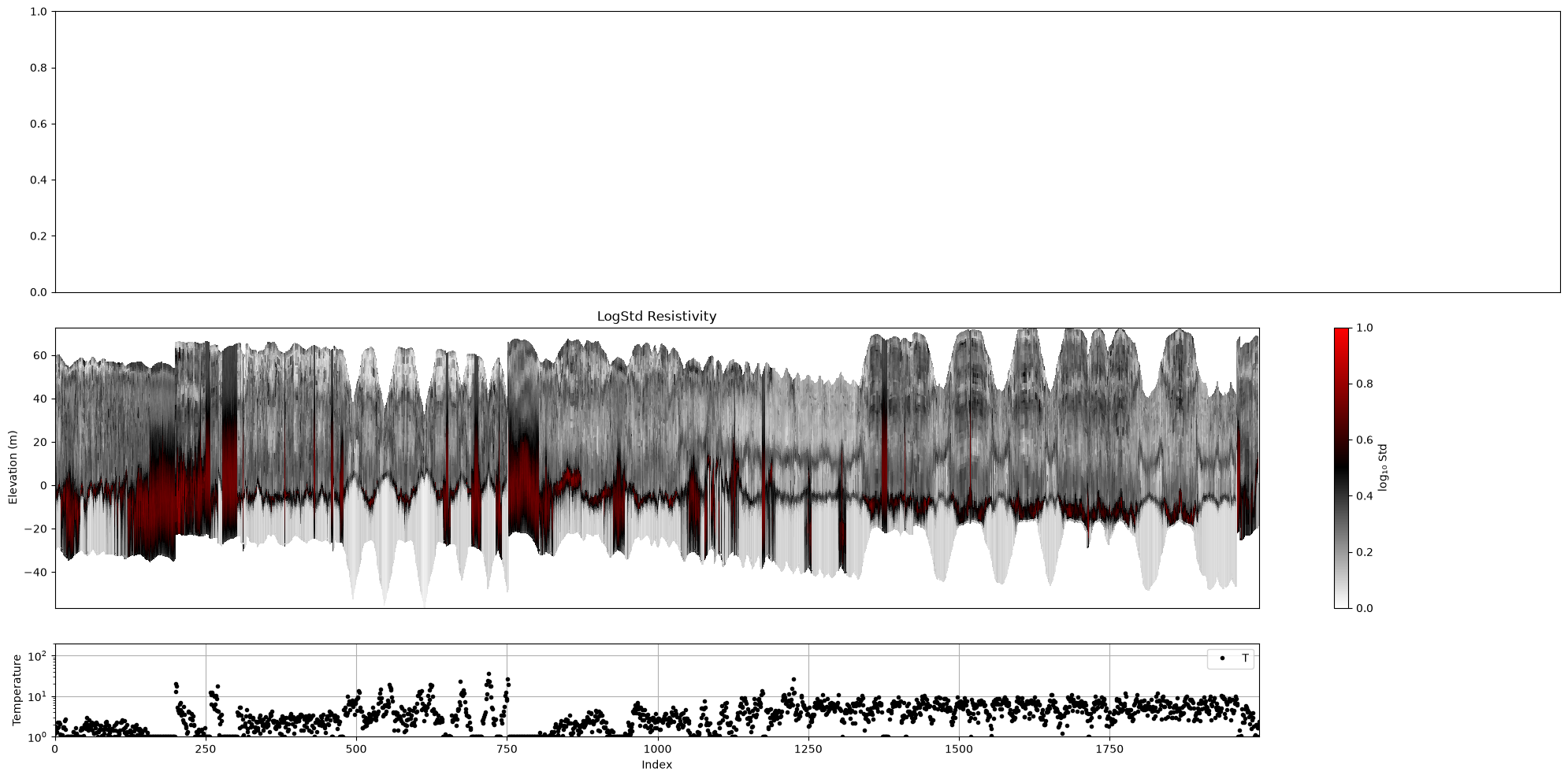
../_images/notebooks_integrate_getting_started_posterior_only_16_3.png

Profile¶

Plot a profile of posterior statistics of model parameters 1 (resistivity)

[10]:

ig.plot_profile(f_post_h5, i1=1, i2=2000, im=1, hardcopy=hardcopy)

Getting cmap from attribute
Warning: HarmonicMean not found in file. Run integrate_posterior_stats() first.

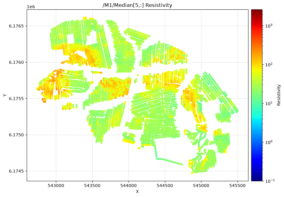
Plot 2d Features¶

First plot the median resistivity in layers 5, 30, and 50

[11]:

# Plot a 2D feature: Resistivity in layer 10
try:
    ig.plot_feature_2d(f_post_h5,im=1,iz=5, key='Median', uselog=1, cmap='jet', s=10,hardcopy=hardcopy)
    plt.show()
except:
    pass

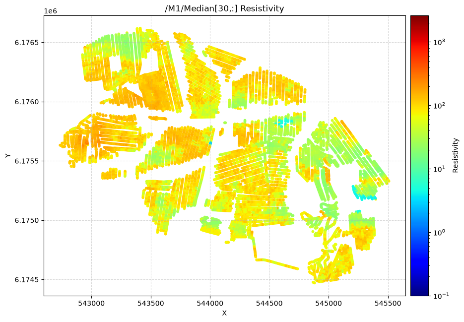
try:
    ig.plot_feature_2d(f_post_h5,im=1,iz=30, key='Median', uselog=1, cmap='jet', s=10,hardcopy=hardcopy)
    plt.show()
except:
    pass

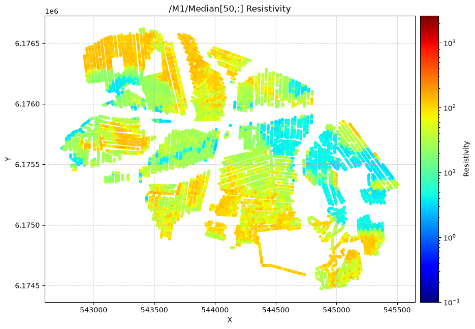
try:
    ig.plot_feature_2d(f_post_h5,im=1,iz=50, key='Median', uselog=1, cmap='jet', s=10,hardcopy=hardcopy)
    plt.show()
except:
    pass

/M1/Median[5,:] Resistivity

../_images/notebooks_integrate_getting_started_posterior_only_20_1.png

/M1/Median[30,:] Resistivity

../_images/notebooks_integrate_getting_started_posterior_only_20_3.png

/M1/Median[50,:] Resistivity

../_images/notebooks_integrate_getting_started_posterior_only_20_5.png

Export to CSV format¶

[12]:

f_csv, f_point_csv = ig.post_to_csv(f_post_h5)

Writing to POST_DAUGAARD_AVG_prior_detailed_general_N2000000_dmax90_TX07_20231016_2x4_RC20-33_Nh280_Nf12_Nu2000000_aT1_M1.csv
----------------------------------------------------
Creating point data set: Median
Creating point data set: Mean
Creating point data set: Std
- saving to : POST_DAUGAARD_AVG_prior_detailed_general_N2000000_dmax90_TX07_20231016_2x4_RC20-33_Nh280_Nf12_Nu2000000_aT1_M1_point.csv

[13]:

# Read the CSV file
#f_point_csv = 'POST_DAUGAARD_AVG_PRIOR_CHI2_NF_3_log-uniform_N100000_TX07_20231016_2x4_RC20-33_Nh280_Nf12_Nu100000_aT1_M1_point.csv'
import pandas as pd
df = pd.read_csv(f_point_csv)
df.head()

[13]:

	X	Y	Z	LINE	Median	Mean	Std
0	543822.9	6176069.6	58.32	140.0	18.622543	24.517012	0.340569
1	543822.9	6176069.6	57.32	140.0	18.622543	19.759150	0.219507
2	543822.9	6176069.6	56.32	140.0	18.241245	17.422058	0.054911
3	543822.9	6176069.6	55.32	140.0	18.622543	17.760700	0.062353
4	543822.9	6176069.6	54.32	140.0	18.360731	17.566660	0.063685

[14]:

# Use Pyvista to plot X,Y,Z,Median
plPyVista = False
if plPyVista:
    import pyvista as pv
    import numpy as np
    from pyvista import examples
    #pv.set_jupyter_backend('client')
    pv.set_plot_theme("document")
    p = pv.Plotter(notebook=True)
    p = pv.Plotter()
    filtered_df = df[(df['Median'] < 50) | (df['Median'] > 200)]
    #filtered_df = df[(df['LINE'] > 1000) & (df['LINE'] < 1400) ]
    points = filtered_df[['X', 'Y', 'Z']].values[:]
    median = np.log10(filtered_df['Mean'].values[:])
    opacity = np.where(filtered_df['Median'].values[:] < 100, 0.5, 1.0)
    #p.add_points(points, render_points_as_spheres=True, point_size=3, scalars=median, cmap='jet', opacity=opacity)
    p.add_points(points, render_points_as_spheres=True, point_size=6, scalars=median, cmap='hot')
    p.show_grid()
    p.show()

[ ]:

[ ]:

[ ]: